
Several months back, I wrote a post about writing code to solve Sudoku puzzles. The point of the article was to illustrate that (in most if not all cases) if you don’t understand a problem, you’re going to struggle to find an appropriate solution. Although I did end up with a partially working app that could find solutions to some puzzles using a brute force approach with backtracking (on github here), what I learned about Sudoku puzzles is that they can easily be solved if addressed as an Exact Cover problem.
The regular puzzle solving approach to solving a Sudoku puzzle is to look at it in terms of the 9×9 grid with some given clues already placed and then try to fill the blanks following the rules of the game, cross-checking that your solution is valid. As a casual player of these puzzles, this is how you would normally play, but it’s not the most efficient approach mathematically. Instead, as an Exact Cover problem, any Sudoku puzzle can be defined as:
- a set of constraints that define the rules of the puzzle
- a finite set of constraints that must be met for a complete solution
- a finite set of all possible candidate values
When a subset of possible candidate values are selected from the set of all possible candidate values that exactly meet all of the constraints once with no unmet constraints, this subset represents a valid solution. There can be more than one solution, although a ‘proper’ Sudoku puzzle is defined as one for which there is only a single, unique solution.
The 4 constraints that must be met for every cell are:
- A single value in each cell
- Values 1 through 9 must exist only once in each row
- Values 1 through 9 must exist only once in each column
- Values 1 through 9 must exist only once in each square
A square (or region) is a 3×3 square – in a 9×9 grid there are 9 total squares, 3 across and 3 down.
For a 9×9 grid using numbers 1 through 9, there are:
9 rows x 9 columns x 9 (values 1 through 9) = 729
… possible candidate values for the cells.
For 4 constraints applied to every cell in the 9×9 grid, there are
9 rows x 9 columns x 4 constrains = 324
… constraints to be met.
A grid of 729 candidate solution rows by 324 constraint columns can be constructed that represents the entire puzzle. An Exact Cover solution is when a subset of the 729 rows is selected that satisfied all of the 324 constraint columns.
This matrix for Exact Cover problems can be represented as a ‘sparse matrix’ where only the cells for each row that correspond to meeting a constraint need to be tracked. The rest of the cells are not relevant and are omitted. This means for each row, there are only 4 cells out of the 324 that need to be tracked in the matrix – the matrix is mostly empty even though a complete grid of 324×729 would be a fairly large table of cells.
Knuth’s paper here observes that by removing (covering) and replacing (uncovering) links to adjacent cells in this matrix is a simple approach to remove rows from the matrix as they are considered as part of the solution and then insert them back into the matrix if a dead end is reached and alternative solutions need to be considered. This approach is what Knuth calls ‘Dancing Links’ as cells are covered and uncovered. The part that makes this approach interesting is that as a cell is covered/removed, the adjacent cell links are updated to point to each other which unlinks the cell in the middle, but the unlinked cell still keeps it’s own links to the adjacent cells to the cell and allows it to easily be inserted back into the linked matrix when the algorithm backtracks to find other solutions.
Many other articles have been written about how the Dancing Links algorithm works, so I won’t attempt to explain this approach in any more detail. Check out Knuth’s paper or any of the other articles linked below. The diagram that is shown in most of these other articles gives a great visual representation of the nodes linking and unlinking.
Implementing the DancingLinks approach in Java
Here’s a brief summary of my working implementation of Dancing Links and Algorithm X, you can grab the full source here on github too.

To represent each cell in the sparse matrix, I created a Class that has up, down, left and right references. As the sparse matrix is generated, each cell inserted into the matrix where a candidate solution row satisfies a constraint column, the cell is inserted with links to each of it’s neighbor cells. Since the linked lists between cells are circular, I believe the term for this data structure is a toroidal doubly-linked list. getters and setters for each of these are used in the cover() and uncover() operations.
The approach to cover and uncover is key for the algorithm to work correctly, as the steps to uncover must be the exact reverse of the steps to cover.
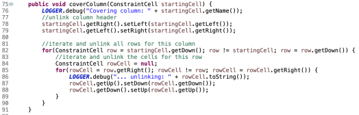
Here’s my cover() :
And here’s my uncover() :

Knuth’s paper defines Algorithm X to solve Exact Cover problems as follows:

The second line, choose a column object, I found out has considerable impact on the performance of this algorithm. Naively, if you just select the next available column in sequence, this would be the simplest approach, but this causes the algorithm to backtrack excessively when finding solutions. I’m not sure exactly why this is, but Knuth’s paper mentions to deterministically select a column. Most suggestions are to do this by selecting the next column that has the least number of remaining solutions left. The impact of these different approaches is interesting, and something I may experiment with more.
Here’s the main section of my implementation of Algorithm X:

The version committed to the github repo has additional inline comments highlighting which parts correspond to the lines in the original pseudo code. For the most part though, this is a line for line implementation of the pseudo code for the algorithm in Knuth’s paper. That’s not that interesting in itself, many have implemented this before. What I found incredibly interesting though was what I learned from coding this.
Lessons Learnt from Implementing Knuth’s Dancing Links and Algorithm X
You would think that given the pseudo code, you could easily code this in an hour or so and have it working. Well, yes to the code it it an hour part, but no to having it working.
What I discovered from attempting to get this working, was that even given what seems like a trivial algorithm, there is plenty that can go wrong. And go wrong it did, catastrophically. I had everything from NullPointerExceptions in my cover() and uncover() (because I hadn’t built the links in my sparse matrix correctly), to StackOverflowErrors from the recursive calls continually calling itself recursively until I exhausted the stack. I had numbers appearing multiple times where they shouldn’t, and some cells with no values at all.
Following my assertion that if you don’t understand a problem you won’t be able to find a reasonable solution, it’s also holds true that if you don’t understand what results you’re expecting, you’re going to struggle to fix it when it doesn’t work.
Debugging recursive algorithms that call themselves deeply and have both logic when the function is called as well as logic that executes on the return are tricky to debug. In this case, the algorithm covers columns as it is called, and uncovers columns when it returns (if a deadend is reached and the algorithm backtracks to find alternative solutions). I found that it was far easier to debug through the first couple of nested calls and check the expected state of the sparse matrix than it was to attempt to debug through to even several levels of nested recursive calls.
I also discovered at the point where I had the majority of the algorithm coded but not yet working, rather than attempt to debug running against a 9×9 grid, a 3×3 grid was far more manageable to step through and examine the state of the matrix. A 3×3 grid has 3 columns, 3 rows, numbers 1 through 9 and a single square. I used constants to define the size of the puzzle, and once the algorithm worked for a 3×3 grid it worked the same for 9×9 (with 9 squares vs 1 for the 3×3 grid).
I used extensive logging in my code, something I would not normally do to the extent that I did here, I normally prefer to step through interactively. Given that the sequence of cell unlinking and linking is essential to the algorithm working correctly, if I put a break point at a step like the cover() method, I could pause at that step and step the sequence of debug output statements to confirm that when column x was covered, it resulted in the expected cells being unlinked during the cover.
JUnit unit tests were invaluable to test each method as I went. The helped build confidence that if I already knew methods a and b were working as expected for example, it highlighted that an issue was elsewhere. It also helped immensely to understand what the expected results were at each stage. If I didn’t understand what the expected results were for a particular step of the algorithm, I read around to understand more, and then wrote my tests to confirm the code was producing the expected results. An interesting side benefit of having working tests along the way, was if I was unsure what the relevance was of a particular part of the algorithm, I could make a change in the code and see if it impacted the results or not by seeing the tests fail. This was useful to understand the behavior of the algorithm.
Comparing my Brute Force Approach with the Knuth Algorithm X and Dancing Links Approach
Taking the same starting puzzle, my previous approach finds a solution in about 50ms on my i7 MacBook Pro. With the new approach using Knuth’s Algorithm X and Dancing Links? 2ms
That’s an incredible difference, just from using a more efficient approach. Is it worth it though?
It depends.
If you’re working on something mission critical where every millisecond counts, then sure, it’s worth it. However, the overhead of understanding a more complex approach, regardless of how much better it runs in practice, comes with a cognitive cost. The effort to understand how the algorithm works takes a non-trivial investment in time and grey cells. If this were code developed for a production enterprise system I would be concerned that other’s could support this code if it failed.
That’s always a valid reason why you should favor simple solutions over more complex ones.
Useful links and other articles
Gareth Threes article: http://garethrees.org/2007/06/10/zendoku-generation/
A Sudoku Solver in Java implementing Knuth’s Dancing Links Algorithm
ScriptingHelpers Dancing Links
An Incomplete Review of Sudoku Solver Implementations
Wikipedia: Soduku, Mathematics of Sudoku, Glossary of Sudoku terms
Hello,
I made a simple Android Java implementation of Algorithm X with links inspired from dancing links (and a non recursive solver). I only used
– right and down links in the nodes
– rowheaders and colheaders with a “cover ID” equal to the current depth level (or 0 if uncovered)
(and so no endless link and relink operations)
– a stack of candidates.
The answer comes in a fraction of a second and I’d like to have your opinion about it (see the Solver class)
Thanks
Here it is:
https://github.com/pc1211/SUDOKU_A
Thanks for the comment, I will take a look at your approach! This interesting thing about Sudoku solvers is that there’s many different approaches, all with their own pros and cons!